Section 3.6 Surfaces
Subsection 3.6.1 Introduction
Most of our lives is not spent in a 2D world (is any of it?), so why would we only look at mathematics in a 2D world? Most of our experiences are three dimensional, so it only makes sense to think about mathematics in a 3D environment.
There are two ways we can visualize a 3D surface. The first way you might consider is having two independent variables, \(x \text{ and } y\text{,}\) and one dependent variable, \(z\text{.}\) So functions of this form are written as
\begin{equation*}
z = f(x,y).
\end{equation*}
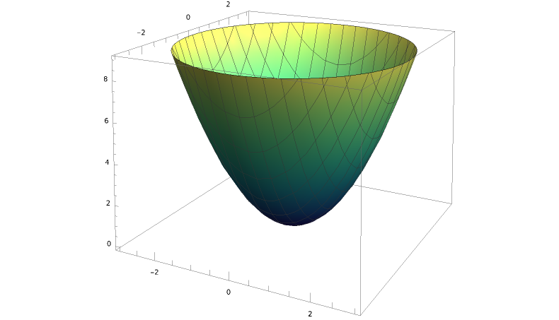
You can see the surface \(f(x,y) = x^2 + y^2\) below.
Subsection 3.6.2 Contour Plots: Connecting 2D and 3D Shapes
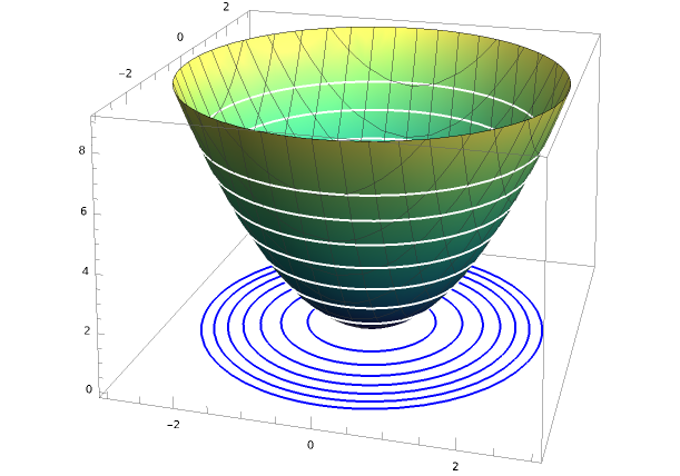
There’s something familiar about \(f(x,y)= x^2 + y^2\text{.}\) Where have you seen something like that before? Well, we know \(x^2 + y^2 = k^2\) is a 2D object: a circle with radius \(k\text{.}\) We so can think of these circles as a part of \(f(x,y) = x^2 + y^2\text{.}\) If you sliced \(f(x,y)\) at height \(k^2\) and put that slice on a plate, the result would be the circle \(x^2 + y^2 = k^2\text{.}\)
These slices are called contours or \(k\)-curves of \(f(x,y)\text{,}\) and each \(k\)- curve of a 3D function results in a 2D object. Keep in mind that when you study explicitly defined functions in the 2D sense, you are actually studying \(k\)-curves of a 3D function.
Subsection 3.6.3 Contour
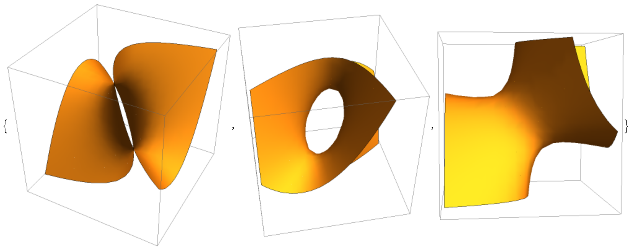
What if there’s some type of mathematical object whose contour is a 3D surface itself? Can you think of how that would work? Yeah, we would need a 4D surface set equal to a constant. That is,
\begin{equation*}
f(x,y,z) = k.
\end{equation*}